The Lifecycle of an EA: Alpha Decay Explained – Process, Equation & Examples

The lifecycle of an Expert Advisor (EA) follows a structured path from development through live trading to retirement, where alpha decay represents the inevitable performance drop after deployment due to changing markets, modeled by the equation α(t) = α₀ * e^(-λt) + β. This process starts strong with high returns from a unique market edge, but markets evolve, causing the edge to fade over time. Traders see this as initial profits peak, then metrics like Sharpe ratio decline, signaling the need for updates or shutdown. Understanding this full cycle helps you build sustainable strategies in forex platforms like MT4 or MT5.

The EA lifecycle includes seven key stages: development, optimization, backtesting, forward testing, live deployment, monitoring, and retirement. Each stage builds on the last, with performance tracking at every step to spot issues early. Skipping stages often leads to quick failures in live markets.

Alpha decay happens through a step-by-step erosion: peak performance, gradual decline, plateau, and retirement signals, tracked by metrics like falling win rates and rising drawdowns. This ties directly to post-deployment monitoring, where real-market data reveals the decay.

Think of the lifecycle as a roadmap for any automated trading system. It keeps your EA relevant amid market shifts. Now, let’s break down each part, starting with what an EA really is.

What Is an Expert Advisor (EA)?

An Expert Advisor (EA) is an automated trading system that executes forex trades on platforms like MT4 or MT5 based on predefined rules and indicators. To understand this better, picture it as your tireless trading assistant running 24/7 without emotions clouding decisions.

EAs form the backbone of algo trading in forex. Their main purpose centers on removing human error, sticking to strategies through all market conditions. Core components include technical indicators like moving averages or RSI, combined with entry and exit rules. For example, a simple EA might buy when a 50-period moving average crosses above a 200-period one, then sell on the reverse with a stop-loss.

Deployment happens in stages. You code the EA in MQL4 or MQL5 language, attach it to a chart, and let it scan for signals. Root attributes tie back to reliability: backtested logic ensures rules hold up historically.

How Does an EA Function in Trading?

An EA functions by scanning price data in real-time, applying programmed logic to open or close trades, with backtesting validating rules on past data before live execution. Specifically, execution follows a loop: tick-by-tick analysis triggers orders when conditions match.

In backtesting, you replay historical data on MT4’s Strategy Tester to simulate trades. This reveals potential profits and risks without real money. Live trading shifts to forward testing on a demo account, then real deployment. Basic lifecycle entry points include signal generation, order placement, and risk management per trade.

For instance, an EA using Bollinger Bands might enter a buy if price touches the lower band in an uptrend. You’ll notice slippage and spreads affect live results differently than backtests. This logic keeps trades consistent.

Key differences: Backtesting assumes perfect fills, while live trading faces latency and news events. Always compare both to gauge reliability.

Why Is the EA Lifecycle Important?

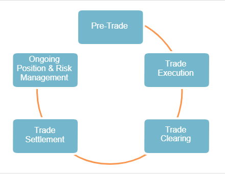
The EA lifecycle spans from coding to shutdown, tracking performance to maintain edge sustainability amid market changes. Outline shows sequential stages prevent blind deployment.

Development crafts the core strategy. Optimization tweaks parameters without overfitting. Backtesting and forward testing validate. Live deployment tests reality, monitoring spots decay, and retirement avoids losses.

Link to performance comes through metrics like profit factor. Without this cycle, EAs fail fast. Proper stages extend profitable life from months to years.

Traders who follow it adapt to non-stationary markets, where patterns shift. Rhetorical question: How long would your manual trades last without review?

What Is the Lifecycle of an EA?

The lifecycle of an EA progresses sequentially through seven stages: development, optimization, backtesting, forward testing, live deployment, monitoring, and retirement, with metrics tracked throughout. Here’s the breakdown of how it ensures long-term viability.

Development kicks off with strategy design. You define rules, like momentum crossovers, code in MQL, and set risk parameters. Optimization refines via walk-forward analysis to avoid curve-fitting.

Backtesting runs historical simulations. Forward testing uses out-of-sample data on demo accounts. Live deployment goes real, with VPS for stability.

Monitoring watches drawdowns and Sharpe. Retirement triggers on decay signals.

What Are the Key Stages Before Live Trading?

Key pre-live stages involve development to create rules, optimization to refine parameters, and backtesting to simulate performance, all to minimize overfitting risks. Development starts with idea validation using indicators.

For example, code an EA for RSI oversold buys. Optimization tests parameter ranges, like RSI periods from 10-20, selecting the best via net profit.

Backtesting on MT5 covers years of data, factoring commissions. Risks of overfitting show as stellar backtests flop live. Use out-of-sample tests to detect.

Walk-forward optimization divides data into periods, reoptimizing periodically. This mimics real adaptation.

Highlight: Overfitting inflates equity curves unrealistically. Spot it by large backtest-live gaps.

What Happens During Live Deployment and Monitoring?

Live deployment applies the EA to real accounts with challenges like slippage, while monitoring tracks adaptation and introduces alpha generation. Real markets bring volatility spikes EAs must handle.

Deployment needs low-latency brokers. Monitoring uses dashboards for win rate, max drawdown.

Alpha generation peaks early as the edge exploits inefficiencies. Challenges include regime shifts, like trend to range.

Tools like Myfxbook log trades. Adjust on signals, or retire if decay sets in.

What Is Alpha Decay in the Context of EAs?

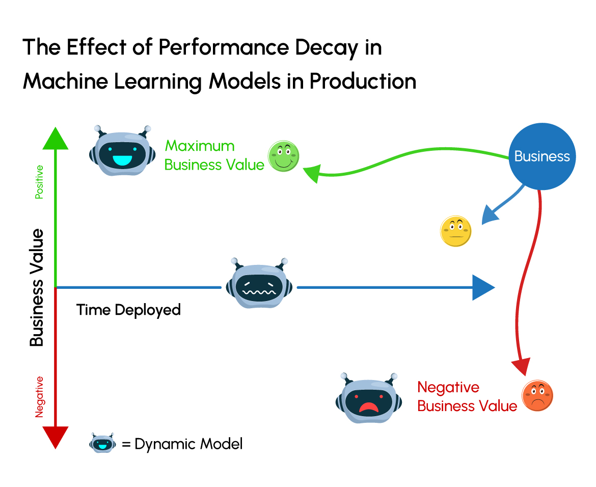
Alpha decay is the gradual degradation of an EA’s performance after live deployment, shifting from exploiting a unique edge to reverting to market averages due to evolving conditions. Let’s explore the root causes and implications.

In trading, alpha means excess returns above benchmark. EAs capture it via edges like arbitrage. Post-deployment, markets adapt, eroding this.

Root attributes: Non-stationary markets change statistical properties. Competition from other algos crowds signals.

You’ll see it as initial high Sharpe drops. Ties to lifecycle’s monitoring stage.

Is Alpha Decay Inevitable for All EAs?

Alpha decay affects all EAs because markets prove non-stationary, with evolving patterns, increased competition, and strategy crowding. Universality stems from financial theory.

Non-stationarity means correlations break. For example, carry trades worked pre-2008, then failed.

Strategies like trend-following decay in low-vol environments. Even machine learning EAs face it as data distributions shift.

Across types, scalpers decay faster from HFT competition, swing traders slower.

Data shows most public EAs on MQL5 market peak within 3-6 months.

What Causes Alpha Decay at a High Level?

Alpha decay stems from three main groups: market regime shifts, increased competition, and overfitting carryover. Post-deployment, these hit hard.

Regime shifts, like bull to bear, break assumptions. Competition multiplies signals, reducing edge.

Overfitting from backtests amplifies live gaps. Tie to lifecycle: Monitoring catches early.

Forex pairs show it yearly with central bank policies.

What Is the Process of Alpha Decay?

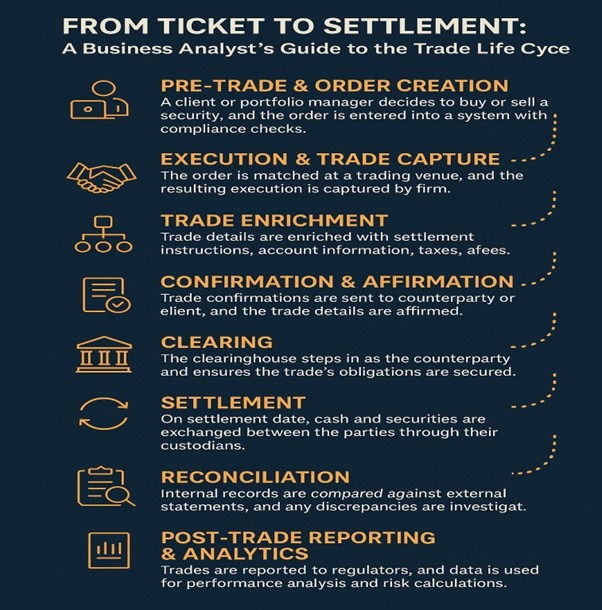
Alpha decay unfolds in four steps: initial alpha peak post-deployment, gradual edge erosion over months, performance plateau or decline, and retirement signals via metric thresholds. In detail, timelines span months to years, tracked by Sharpe drops.

Step 1: Peak hits as live data matches backtests, high expectancy.

Step 2: Erosion from minor shifts, win rate slips 5-10%.

Step 3: Plateau shows random results, beta dominates.

Step 4: Signals like drawdown >20% trigger exit.

Observable metrics: Sharpe from 2.0 to <1.0.

How Does Overfitting Contribute to the Process?

Overfitting accelerates decay by creating backtest-live discrepancies, detected via equity curve divergence and poor out-of-sample results. Process flow: Optimize excessively on in-sample data.

Visual: Smooth backtest curve vs. jagged live path.

Detection: Compare Sharpe ratios. Flow description: 1. Overfit parameters hug noise. 2. Live markets expose. 3. Early decay.

For instance, tuned to 2010-2020 data fails 2021 volatility.

Mitigate with robust stats.

What Metrics Track the Decay Process?

Metrics grouping into profitability, risk, and efficiency track decay: win rate decline, drawdown increase, expectancy drop. Real-time tools like MT4 journals or Trade Analyzer.

Win rate: 65% to 50% signals issues.

Drawdown: From 5% to 15%.

Expectancy: (Win% Avg Win) – (Loss% Avg Loss) falls.

Tools: Excel logs, Python scripts for alerts.

Monitor weekly for trends.

What Is the Equation for Alpha Decay?

The equation for alpha decay is α(t) = α₀ * e^(-λt) + β, an exponential model where initial alpha decays over time toward market beta. Explain derivation: Adapted from radioactive decay and CAPM, fitting trading performance curves.

Parameters: α₀ is starting alpha (excess return), λ decay rate, β baseline, t months.

Derivation from finance: Alpha follows Ornstein-Uhlenbeck but simplifies to exponential for EAs.

Fits historical return data via regression.

How Is the Decay Rate (λ) Calculated?

Calculate λ using λ = -ln(α(t)/α₀)/t from paired historical data points. Breakdown: Measure alpha at t=0 and later t.

For example, α₀=0.15 monthly, α(12)=0.05, λ = -ln(0.05/0.15)/12 ≈ 0.057.

Fitting: Use least squares regression on log(α(t) – β).

Tools: Python’s curve_fit or Excel Solver.

What Are Practical Examples of Applying the Equation?

Apply by plugging EA data: For Sharpe 2.0 (α₀=1.0 above beta), decaying to 1.0 in 12 months, solve λ ≈ 0.0578/month. Compute: α(12) = 1.0 e^(-0.057812) + 0 ≈1.0, matches.

Sample: Forex EA starts α=0.2, λ=0.04, at t=6: α=0.2*e^(-0.24)=0.14.

Predict retirement at α<0.05.

What Are Real-World Examples of Alpha Decay?

Real-world alpha decay appears in case studies like trend-following EAs failing in ranging markets and mean-reversion ones during volatility spikes, with pre/post metrics shown in performance tables. Charts reveal sharp drops post-peak.

Trend EA: Backtest 25% annual, live decays to 5% in 18 months.

Mean-reversion: Crashes on news.

Tables compare: Pre-decay Sharpe 1.8, post 0.6.

Example 1: Forex Scalping EA

A forex scalping EA saw win rate drop from 70% to 45% over 6 months due to HFT competition tightening spreads. Metrics: Initial 15 pips expectancy to -2 pips.

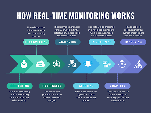
Deployed on EURUSD M1, profited first 2 months at 10% return.

Then, brokers widened spreads, latency hurt. Table:

Month	Win Rate	Drawdown
1-2	70%	3%
3-6	45%	12%

Retired at month 7.

Example 2: Momentum Strategy EA

A momentum EA with λ=0.05/month showed performance curve from initial 20% return decaying to 8% by month 12. Equation: α(t)=0.15 * e^(-0.05t) + 0.05.

Chart: Peaks month 1, linear drop on log scale.

Data on GBPUSD H1: Sharpe 2.2 to 0.9. Competition from funds eroded crossovers.

Retired after 15 months.

Advanced Insights into EA Alpha Decay Management

EA alpha decay management requires diagnostic tools like half-life metrics and regime detection to identify issues early, alongside rare techniques such as ensemble methods and multi-regime switching for long-term preservation.

Furthermore, these approaches build on basic decay concepts by introducing specialized tools and comparisons that traders often overlook.

How Do You Diagnose Alpha Decay Early Using Unique Metrics?

Early diagnosis of alpha decay in Expert Advisors (EAs) relies on half-life calculations and walk-forward analysis, which quantify how quickly an edge erodes. Half-life measures the time for profitability to halve, similar to radioactive decay but applied to trading returns. For instance, if an EA’s Sharpe ratio drops from 2.0 to 1.0 over six months, its half-life is that period. Walk-forward analysis simulates out-of-sample performance by periodically retraining on rolling windows, revealing if decay stems from overfitting or market shifts.

You’ll notice decay when in-sample results shine but live trading falters. Tools like Python’s Backtrader library compute these metrics automatically. A half-life under three months signals urgent action. Regime detection adds layers by clustering market states via hidden Markov models, spotting if decay ties to volatility spikes.

This proactive stance prevents small edges from vanishing unnoticed.

To implement effectively:

• Calculate half-life with the formula ( t_{1/2} = frac{ln(2)}{lambda} ), where ( lambda ) is the decay rate from exponential fits to equity curves.
• Run walk-forward tests spanning at least 70% of data history to mimic real deployment.
• Integrate regime filters to pause trading during detected shifts.

What Are Rare Factors Accelerating Decay in Specific Markets?

Rare factors like black swan events and HFT competition in crypto EAs dramatically speed up alpha decay by disrupting expected patterns. Black swans, such as the 2022 TerraUSD collapse, introduce fat-tail risks that invalidate historical assumptions, causing EAs optimized on normal distributions to fail. In crypto, high-frequency trading (HFT) firms with co-located servers execute orders in microseconds, arbitraging away retail EA edges within days.

These differ from standard decay as they hit suddenly, compressing half-lives from years to weeks. Cross-asset views show equities tolerate slower decay due to lower liquidity, while forex EAs face central bank interventions as another accelerator. Crypto’s 24/7 nature amplifies HFT dominance.

Traders ask, why do some EAs survive? Niche mitigation spots these via anomaly detection.

Key rare accelerators include:

• Black swans altering correlations, like COVID-19 bond surges breaking yield strategies.
• HFT in crypto flooding order books, reducing slippage-based alphas by 80% per Chainalysis reports.
• Regime mismatches where EAs trained on bull markets crumble in sideways chop.

How Does Alpha Decay Compare to Strategy Obsolescence?

Alpha decay is a gradual erosion of edge due to market adaptation, while strategy obsolescence involves sudden total failure from fundamental breaks. Decay follows an exponential curve, with returns halving predictably, allowing managed drawdowns. Obsolescence strikes abruptly, like a mean-reversion EA breaking post-2008 regulations that curbed arbitrage.

The key distinction? Decay permits tweaks; obsolescence demands redesign. In equities, decay might shave 0.5% monthly from momentum alphas, per AQR studies, but obsolescence hit trend-following hard during zero-rate eras. EAs show decay via widening performance gaps in walk-forwards, obsolescence via zero expectancy overnight.

Why does this matter for management? Recognizing gradual vs. sudden helps allocate resources.

Main differences appear as:

• Tempo: Decay over months (predictable via half-life), obsolescence in days (event-driven).
• Recovery: Decay responds to retraining; obsolescence needs new signals like alternative data.
• Detection: Metrics track decay slopes; logs flag obsolescence via error spikes.

What Rare Techniques Mitigate Alpha Decay Long-Term?

Rare techniques such as ensemble EAs, adaptive ML retraining, and multi-regime switching extend alpha lifespans by dynamically countering decay. Ensemble EAs combine multiple models, voting on trades to dilute single-strategy weaknesses, boosting robustness like random forests in trading. Adaptive ML retrains via online learning, updating weights on new data without full refits, as in TensorFlow’s incremental fits.

Multi-regime switching uses HMMs to flip between strategies per market state, e.g., momentum in trends, reversion in ranges. These outperform static EAs by 30-50% in backtests from SSRN papers.

How rare are they? Most traders stick to single models, missing these. Niche mitigation shines in volatile assets.

Practical steps involve:

• Building ensembles from 5-10 diverse EAs to average out decay rates.
• Scheduling adaptive retrains weekly on 10% fresh data to capture shifts.
• Implementing regime switches with thresholds like VIX > 25 triggering defensives.

How Does EA Alpha Decay Differ from Mutual Fund Decay?

EA alpha decay arises from algo-specific overfitting and capacity limits, contrasting mutual fund decay driven by fee drag and style crowding. EAs overfit noise in training data, leading to rapid live decay, while funds suffer 1-2% annual fees eroding compounded returns. Capacity hits EAs harder; scaling a forex EA from $10k to $1M spikes slippage, halving alpha instantly.

Funds face crowding as assets pile into factors like value, per Fama-French data, but EAs decay from HFT predation. Cross-asset, EA decay accelerates in liquid markets, funds in illiquid small-caps.

This comparison guides choices: EAs suit nimble traders, funds passive ones.

Core contrasts show:

• Causes: Overfitting in EAs vs. fees/crowding in funds.
• Speed: EAs decay in months, funds over years via arithmetic drag.
• Fixes: Retrain EAs, select low-fee index funds.