Understanding Expectancy: What is Mathematical Expectation (Expected Value)?

Mathematical expectation, or expected value, is the long-run average value you get from repeating a random experiment many times. Think of it as the center of gravity for all possible outcomes, weighted by how likely each one is. In probability theory, this concept helps predict average results over endless trials, even if single tries vary wildly. For example, in gambling or insurance, it shows if a game favors the house or the player in the long haul.

Expected value differs from a simple average of observed data. While a sample mean comes from actual results you collect, expected value uses probabilities to forecast the theoretical average. Over many repetitions, your sample averages approach this value, thanks to the law of large numbers. This makes it a powerful tool for decisions under uncertainty.

Expectancy serves as another name for expected value in probability contexts. The term traces back to Jacob Bernoulli in the 17th century, who used it to describe anticipated outcomes in games of chance. Today, both terms mean the same: a probability-weighted average that guides risk assessment.

You might wonder, how does this apply in real life? From stock trading to weather forecasting, expected value underpins choices. Now, let’s break it down step by step, starting with its core definition.

What Is Mathematical Expectation?

Mathematical expectation is a core concept in probability theory defined as the long-run average value of repetitions of an experiment, calculated as a weighted average using probabilities. Specifically, it captures what you can anticipate on average from a random variable, no matter how unpredictable each trial feels.

In detail, imagine flipping a coin 1,000 times. The results jump around, but the average settles near the expected value. This idea forms the backbone of statistics and decision-making. Probability theory treats random variables—functions mapping outcomes to numbers—like heights or test scores in a population. The expected value, denoted E[X], sums each possible value times its probability.

You’ll notice this weighted average differs from arithmetic means. If outcomes are equally likely, it matches the regular average. Otherwise, rarer big wins or losses pull it accordingly. For instance, a lottery ticket costs $1 with a tiny chance of millions. The expected value stays negative, explaining why lotteries profit operators.

Root attributes make it fundamental. It ignores variance, focusing solely on central tendency. This linearity property, which we’ll cover later, lets you break complex problems into simpler parts. In practice, engineers use it for reliability predictions, economists for market models.

Why does this matter to you? It shifts focus from luck to long-term patterns. A fair six-sided die has expected value 3.5, so rolling it often yields about $3.50 per roll if paid face value. Casinos design games with negative expectation to win over time.

Let’s clarify common mix-ups. People often confuse it with most likely outcomes. No, it’s the balance point. In continuous cases, like waiting times, it integrates over densities. Historical roots from Bernoulli formalized it in Ars Conjectandi (1713), bridging games to science.

Is Expected Value the Same as the Average?

No, expected value is not the same as the average, though the long-run average of many trials converges to it; the key difference lies in probabilities versus observed data. The sample mean uses actual results, while expected value relies on theoretical probabilities.

For example, suppose you roll a die 10 times and get an average of 4.2. That’s your sample mean, varying with luck. Repeat 10,000 times, and it nears 3.5, the expected value. This convergence follows the law of large numbers, a theorem proving averages stabilize.

The sample mean, bar{X} = (sum of observations)/n, reflects finite data. It can mislead with small samples. Expected value E[X] = sum x_i P(X=x_i) stays fixed, immune to chance. Statisticians estimate E[X] from samples but know it’s an approximation.

Consider a biased coin landing heads 60% of the time, heads worth 1 point, tails 0. Expected value is 0.6, but three flips might average 0, 1, or whatever. Long-run flips average 0.6.

Benefits appear in applications. In quality control, expected defect rates guide production. Observed averages fluctuate; expected values set targets. Research from Feller’s Introduction to Probability shows this distinction prevents errors in hypothesis testing.

You’ll see it in finance too. Stock returns’ sample averages from past data approximate expected returns, but models use probabilities for forecasts. This clarity aids better investing.

What Does Expectancy Mean in Probability?

Expectancy means the same as expected value: the probability-weighted average of a random variable’s outcomes. Jacob Bernoulli coined it in the late 1600s while studying repeated trials, formalizing ideas from Pascal and Huygens on gambling.

Specifically, Bernoulli’s work showed how averages emerge from chance. His law of large numbers links sample means to expectancy, proving reliability over repetitions. Today, texts use terms interchangeably, but “expectancy” evokes anticipation.

For instance, in insurance, expected claims per policy set premiums. If average payout is $100 with probability 0.1, expectancy is $10, plus costs for profit.

Historical context enriches it. Bernoulli’s Ars Conjectandi solved the “St. Petersburg paradox,” where infinite expectancy clashes with finite bets people make. This highlighted utility over raw value, influencing economics.

In modern probability, expectancy quantifies risk. Heavy-tailed distributions like Cauchy lack it, as integrals diverge. Conditions include finite variance or absolute integrability.

Evidence from Kolmogorov’s axioms solidifies it. Probability spaces define random variables, and expectancy extends to functions via linearity.

How Do You Calculate Expected Value for Discrete Random Variables?

Calculate expected value for discrete random variables using E[X] = Σ x_i * P(X = x_i) over all possible outcomes, yielding the probability-weighted average in a few steps. Here’s the breakdown for precise computation.

First, identify all possible values x_i and their probabilities P(X = x_i), ensuring they sum to 1. Multiply each x_i by its probability, then sum results. This formula handles countable outcomes like coin flips or card draws.

Step-by-step process:

1. List distinct outcomes and assign probabilities.

2. Compute x_i * P(X = x_i) for each.

3. Add them up for E[X].

Take a game paying $2 on even die rolls (probability 0.5), $4 on 3 (1/6), nothing else. E[X] = 20.5 + 4(1/6) + 0*(0.5) = 1 + 0.666 = 1.666. Positive value means player edge.

Root attributes shine in discrete cases. Finite or countably infinite supports work if sum |x_i| P_i converges. Computers sum large lists easily.

Why step-by-step? It avoids errors. For joint variables, marginalize first. In Poisson processes, like customer arrivals, E[X] = λ, the rate.

Practice with lotteries. Powerball jackpot $100 million, 1 in 292 million odds, $2 ticket. E[X] ≈ (100e6 / 292e6) – 2 ≈ -1.66. Negative warns against play.

Extensions include indicators. E[I_A] = P(A), simplifying many proofs.

What Is an Example of Expected Value with Dice?

For a fair six-sided die, expected value E[X] = 3.5, computed as (1+2+3+4+5+6)/6 since each face has probability 1/6. Group fair die outcomes: 1 through 6, each equally likely.

Specifically, apply the formula: E[X] = 1(1/6) + 2(1/6) + … + 6*(1/6) = (21/6) = 3.5. This means endless rolls average 3.5.

For evidence, simulate 1,000 rolls: averages hover near 3.5, stabilizing more with trials. Law of large numbers guarantees it.

Visualize a number line; 3.5 balances the bar. Biased dice shift it. If faces 1-5 equal, 6 twice likely, E[X] > 3.5.

Real use: board games like Monopoly use dice expectations for turn lengths. About 3.5 spaces per roll informs strategy.

Compare unfair die: P(6)=0.3, others equal. Recalculate to 3.9, favoring high rolls.

What Is Expected Value for a Coin Flip?

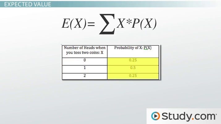
For a fair coin flip with heads paying $1 and tails $0, expected value is 0.5. Simple binary: two outcomes, P(heads)=P(tails)=0.5.

Compute: E[X] = 10.5 + 00.5 = 0.5. Biased coin, P(heads)=0.6, E[X]=0.6.

For payoffs, say heads +$10, tails -$5, fair coin. E[X] = 100.5 + (-5)0.5 = 2.5. Positive suggests play long-term.

Evidence from repeated flips shows convergence. 100 flips average near 0.5.

In betting, martingale systems fail against house edge, as expectation stays negative.

How Do You Calculate Expected Value for Continuous Random Variables?

For continuous random variables, compute expected value with E[X] = ∫_{-∞}^{∞} x f(x) dx, where f(x) is the probability density function. To understand this better, note it generalizes discrete sums to integrals over densities.

The pdf f(x) satisfies ∫ f(x) dx = 1, giving probability P(a < X < b) = ∫_a^b f(x) dx. Expected value weights x by f(x).

Step-by-step:

1. Determine f(x) for the distribution.

2. Set up integral ∫ x f(x) dx over support.

3. Evaluate, often using known formulas.

For exponential distribution f(x) = λ e^{-λx}, x≥0, E[X]=1/λ. Waiting times average 1/λ.

Root attributes: requires ∫ |x| f(x) dx < ∞. Unlike discrete, no point masses.

Normal distribution N(μ,σ²) has E[X]=μ, intuitive mean.

Software like R or Python’s SciPy computes numerically for customs.

Example: rainfall modeled uniform 0-10 cm. See subhead.

Challenges: improper integrals diverge for some, like Cauchy.

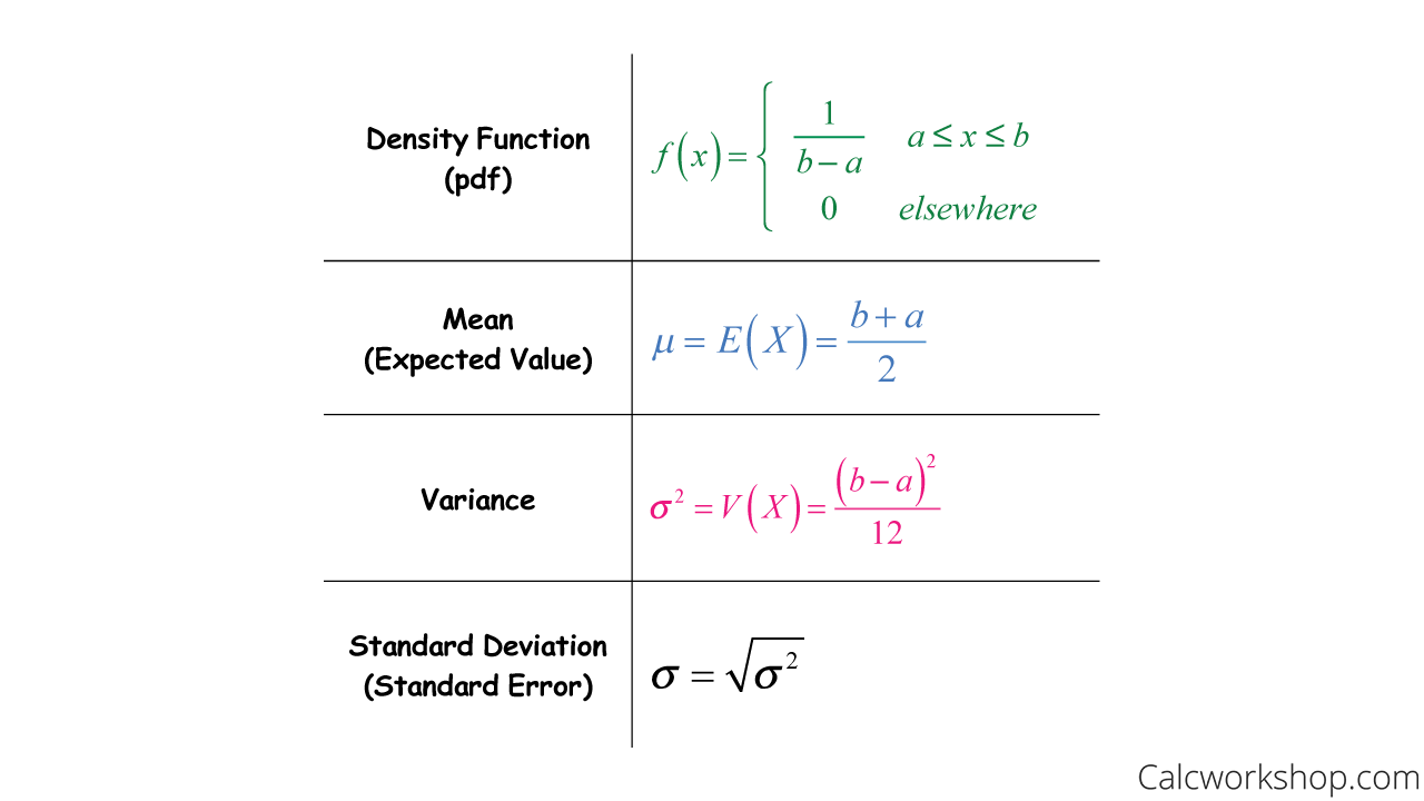
What Is Expected Value for a Uniform Distribution?

For uniform distribution over [a,b], expected value is E[X] = (a + b)/2. Parameters a to b define equal density f(x) = 1/(b-a).

Compute: ∫_a^b x /(b-a) dx = [x²/(2(b-a))]_a^b = (b² – a²)/(2(b-a)) = (a+b)/2.

Visual integration: area under x f(x) triangle peaks midway.

For [0,1], E[X]=0.5. Simulations confirm.

Rainfall [0,10], average 5 cm. Symmetric, midpoint.

Compare triangular: shifts with peak.

What Are the Main Properties of Expected Value?

Main properties include linearity E[aX + bY] = aE[X] + bE[Y], non-negativity for positive variables, and monotonicity if X ≥ Y then E[X] ≥ E[Y]. Let’s explore these algebraic tools.

Linearity holds unconditionally, even if X,Y dependent. Simplifies E[X+Y+Z] = E[X]+E[Y]+E[Z].

Proof: from definitions, integrals or sums distribute.

Non-negativity: if X ≥ 0, E[X] ≥ 0, by weighting positives.

Monotonicity follows similarly.

Other traits: E[c] = c for constants. E[g(X)] needs computation.

Root attributes make it versatile. Tower property E[E[X|Y]] = E[X] for conditioning.

In variance, Var(X)=E[X²] – (E[X])².

Applications: portfolio theory, E[return] = sum weights * E[asset].

Counterexamples: no multiplicativity, E[XY] ≠ E[X]E[Y] unless independent.

Does Expected Value Always Exist?

No, expected value does not always exist for heavy-tailed distributions where ∫ |x| f(x) dx diverges. Conditions demand finite first moment, E[|X|] < ∞.

For Cauchy, f(x)=1/(π(1+x²)), symmetric but tails decay slowly. Integral oscillates, no E[X].

Student-t with 1 degree lacks it; needs >1.

Evidence: Levy stable distributions often finite only for α>1.

Practical note: finance models assume existence, but real markets have fat tails.

Check via moments or simulations diverging.

What Are Advanced Applications and Comparisons of Expected Value?

Expected value extends beyond basics into gambling strategies, insurance pricing, conditional probabilities, utility decisions, and stochastic processes like martingales, differing from variance by measuring central tendency instead of dispersion.

Furthermore, these applications reveal how expected value guides real-world choices under uncertainty.

How Does Expected Value Apply to Gambling and Insurance?

Expected value serves as a core tool in gambling and insurance by quantifying long-run average outcomes per bet or policy. In gambling, players calculate it to assess bet profitability. For a coin flip bet where heads wins $2 and tails loses $1, with fair odds, expected value equals (0.5 2) + (0.5 -1) = 0.5 – 0.5 = 0, marking a fair bet. Casinos ensure a house edge, a negative expected value for players, like 5.26% in American roulette, guaranteeing profits over many plays.

Insurance companies use expected value for premium setting. They estimate claim probabilities and costs, say a 1% fire risk costing $100,000 on average, yielding an expected loss of $1,000 per policy. Premiums exceed this to cover operations and profits, balancing risk pooling.

This approach highlights differences: gambling often seeks positive expected value through edges, while insurance aims for near-zero net expected value after premiums.

You’ll notice gamblers chase short-term variance, but expected value predicts long-term results. Insurance relies on the law of large numbers for accuracy.

To spot value bets, compute expected value from odds and payouts.

Moreover, fair bets have zero expected value, but real scenarios include edges.

• House edge calculations subtract casino advantage from 100% payout odds, like blackjack’s 0.5% edge on basic strategy.
• Fair bets balance wins and losses exactly, encouraging play without long-term drain.
• Actuarial tables refine insurance expected values using historical data for precise pricing.

What Is Conditional Expected Value?

Conditional expected value, denoted E[X|Y=y], measures the average of X given specific Y outcomes, refining predictions under new information. Unlike unconditional expected value, it adjusts for conditions, as in Bayes’ theorem applications.

For example, in weather forecasting, E[rainfall|clouds] might be 0.3 inches versus 0.05 inches unconditionally. The tower property, E[E[X|Y]] = E[X], ensures consistency, averaging conditional values yields the overall expectation.

This form appears in finance for portfolio adjustments given market signals, or medicine for disease probabilities post-tests.

It contrasts with total expected value by incorporating dependencies, vital for sequential decisions.

Let’s see how it builds on basics: start with joint distributions, then condition.

Rhetorical question: what if new data changes everything?

This property underpins advanced modeling.

Additionally, the tower property simplifies nested expectations in proofs.

– E[X	Y=y] uses conditional probability mass functions, summing x * P(X=x	Y=y).
– Tower property proves by iterated expectation, E[E[X	Y]	Z] = E[X	Z].

• Applications include filtering in signal processing, predicting states from observations.

How Does Expected Value Compare to Variance and Standard Deviation?

Expected value captures the mean outcome, while variance measures spread around that mean, and standard deviation is its square root for scale. Expected value, E[X] = sum x P(x), focuses on balance point; variance, Var(X) = E[(X – E[X])^2], quantifies risk or uncertainty.

For a die roll, E[X] = 3.5, but Var(X) ≈ 2.92 shows outcome scatter. A certain $3.5 has zero variance, same mean but no risk.

They complement: high expected value with low variance signals reliable gains, like bonds versus stocks.

Variance ignores direction, penalizing upside and downside equally, unlike expected value’s net focus.

In investments, expected return draws capital, variance demands compensation via risk premiums.

How do they pair in practice? Portfolios optimize mean-variance trade-offs.

This distinction clarifies: mean predicts average, spread predicts fluctuations.

Besides that, standard deviation aids normal distribution interpretations, like 68% within one SD.

• Expected value equals weighted average, central tendency metric.
• Variance decomposes total risk into average squared deviation.
• Standard deviation scales variance for intuitive percentage risks in finance.

What Is the Role of Expected Value in Utility Theory?

In utility theory, expected value evolves into expected utility, where agents maximize E[U(W)], U being a utility function reflecting risk preferences. Von Neumann-Morgenstern axioms justify this, assuming rational choices under lotteries.

Risk-averse individuals, with concave U, prefer certain outcomes over equal expected value gambles, like $50 for sure versus 50% chance of $100. Risk aversion coefficient, -U”/U’, quantifies this.

Expected value assumes linear utility, ignoring attitudes, so expected utility corrects for behavior.

Decision theory uses it for choices: buy insurance despite negative expected value due to high utility loss aversion.

It contrasts monetary expected value by personalizing via utility.

What’s more, prospect theory modifies it with reference points and loss weighting.

This framework explains paradoxes like Allais, where expected value fails.

In particular, it guides portfolio selection under behavioral lenses.

• Von Neumann-Morgenstern requires completeness, transitivity, continuity, independence for expected utility representation.
• Risk aversion leads to Jensen’s inequality, E[U(X)] < U(E[X]) for concave U.
• Applications span economics, from consumer choice to contract design.

How Does Expected Value Relate to Martingales in Stochastic Processes?

Martingales are stochastic processes where E[X_{t+1} | X_1, …, X_t] = X_t, embodying fair game property with constant expected value conditionally. Future expectations equal current value given history.

This zero-drift condition links to expected value: overall E[X_t] stays constant.

The optional stopping theorem bounds gains from stopping rules, preventing arbitrage in fair games.

In finance, stock prices under risk-neutral measure form martingales, pricing derivatives via expected payoffs.

It differs from expected value alone by enforcing conditional fairness sequentially.

Rhetorical question: can you beat a fair game by timing exits?

No, theorems prove limits.

Moreover, supermartingales have decreasing expectations.

This ties to gambling systems failing long-term.

• Fair game property ensures no predictable drift, E[change] = 0 conditionally.
• Optional stopping theorem requires bounded stops or uniform integrability for E[X_tau] = E[X_0].
• Examples include random walks, Polya’s urn, pricing in Black-Scholes model.